Publication Info
- Title:
- Existence of the solution to a nonlocal-in-time evolutional problem
- Type:
- Article
- Status:
- Published
- Journal:
- Nonlinear Anal. Model. Control 19 (3), 432-447
Extended summary
This work is devoted to the study of a nonlocal-in-time evolutional problem for the first order differential equation in Banach space.
\begin{equation} \label{bp1:eq} u’_t + Au=f(t), \quad t \in [0,T] \end{equation}
\begin{equation} \label{bp1:nc} u(0)+\sum\limits_{k=1}^{n}\alpha_k u(t_k) =u_0,\quad 0 < t_1 < t_2 < \ldots < t_n \leq T, \end{equation}
Sufficient conditions guarantying the existence of solution to \eqref{bp1:eq} — \eqref{bp1:nc} was formulated by Byszewski and Liang. According to them the solution of \eqref{bp1:eq} — \eqref{bp1:nc} exists if the coefficients from \eqref{bp1:nc} satisfy the following inequality \begin{equation}\label{estLiang2002} \sum\limits_{i=1}^{n} \left|\alpha_i\right|e^{-\rho t_i} \leq 1. \end{equation}
Our primary approach, although stems from the convenient technique based on the reduction of a nonlocal problem to its classical initial value analogue, uses more advanced analysis. That is a validation of the correctness in definition of the general solution representation given by \begin{equation} \label{bp1IntRed} u(t)=e^{-At} B^{-1} \left[ u_0 - \sum\limits_{i=1}^n \alpha_i \int\limits_0^{t_i} e^{-A (t_i-\tau)}f(\tau) d\tau\right] +\int\limits_0^t{e^{-A(t-\tau)}f(\tau)}d\tau. \end{equation} here $B(z)$ is defined as follows: \begin{equation} \label{zerosExp} B(z)=1+\sum_{k=1}^n{\alpha_k e^{(-t_k z)}}. \end{equation} Such approach allows us to reduce the given existence problem to the problem of locating zeros of a entire function $B(z)$. It results in the necessary and sufficient conditions for the existence of a generalized (mild) solution to the given nonlocal problem:
Theorem 1.
Let $A$ be a strongly positive linear operator with the spectral parameters $(\rho, \theta)$, and $f(t) \in L^1((0;T),X)$ be a given function. Then the generalized solution \eqref{bp1IntRed} exists if and only if the set of zeros $\mathrm{Ker}(B(z)) \equiv \left\{z: B(z)=0,\ z \in \mathbb{C} \right\}$ of $B(z)$ associated with nonlocal condition \eqref{bp1:nc}, satisfy the inclusion \begin{equation}\label{zerosB} \mathrm{Ker}(B(z))\subset \mathbb{C} \backslash \Sigma. \end{equation}
Example 1.
To demonstrate the application of Theorem 1 let us consider the following nonlocal problem \begin{equation} \begin{array}{l} u’_t+Au=f(t), \quad t \in [0,T]\\ u(0)+\alpha_1 u(t_1) =u_0,\quad 0<t_1\leq T. \end{array}\label{exNCP1p} \end{equation} Condition \eqref{zerosB} for problem \eqref{exNCP1p} is equivalent to the following inequality: \begin{equation}\label{estNC1p} \left|\mathrm{Arg}\left(-\frac{1}{\alpha_1}\right)\right|>\left(\ln\left|{\alpha_1}\right|-t_1\rho\right)\tan\theta. \end{equation}
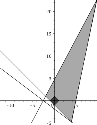
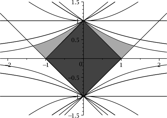
The comparison of sufficient condition \eqref{estLiang2002} against necessary and sufficient condition \eqref{estNC1p} is given on Figure 1 where we depict three sets of admissible values of $\alpha_1 \in \C$ for $t_1=1$: $\cbox{gray80}$ — estimate \eqref{estLiang2002} ($\theta=\pi/4$), $\cbox{gray60}$ — estimate \eqref{estNC1p} ($\theta=\pi/4$) and $\cbox{gray40}$ by estimate \eqref{estNC1p} ($\theta=\pi/6$).
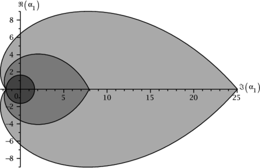
Observe that for the operator $A$ with spectral parameters $(1,\pi/4)$ ($\rho=1$, $\theta=\pi/4$) the set of admissible $\alpha_1$ obtained from \eqref{estNC1p} (interior of the region coloured in $\cbox{gray60}$) contains in itself as a subset the admissible set obtained by \eqref{estLiang2002} (coloured in $\cbox{gray80}$). This set remains the same for the whole family of sectorial operator coefficients with some fixed $\rho$ and $\forall \theta \in [0, \pi/2]$ since \eqref{estLiang2002} are independent of $\theta$. While in reality the admissible set grows larger when we make $\theta$ smaller. Check for example the corresponding set for the case $\theta=\pi/6$ obtained using \eqref{estNC1p} which is coloured in $\cbox{gray40}$ on Figure 1. In the limiting case of $\theta=0$ when $A$ is self-adjoint this set becomes equal to $\C \backslash (-\infty; -e^{t_1\rho})$.
A mapping
\begin{equation}
\label{bp_transf1}
\varphi(z)=\exp(-z/Q), \quad Q=\mbox{LCM}(\mu_1,\mu_2, \ldots, \mu_n)
\end{equation}
transforms \eqref{zerosExp} into the following form
\begin{equation}
\label{zerosPol}
P(z)=1+\suml_{k=1}^{n}\alpha_k z^{c_k}.
\end{equation}
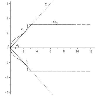
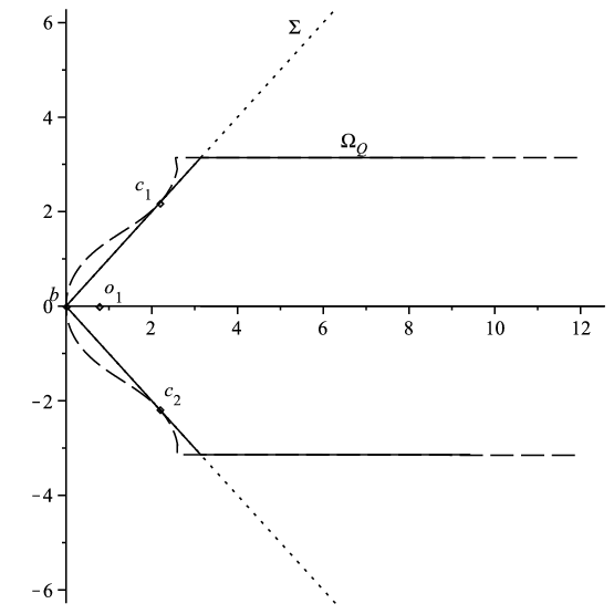
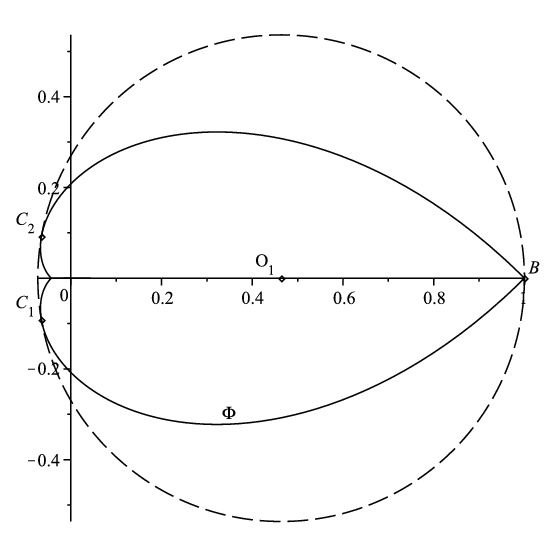
It is well known that \eqref{zerosExp} is one-to-one conformal mapping of $\Omega_Q$ onto $\Phi$ (see Figure 2 b)).

The conditions guarantying that all roots of $P(z)$ lie outside $\Phi$ or equivalently $\Ker{B(z)} \subset D_{Q} \backslash \Omega_Q$ would be necessary and sufficient to prove that existence and uniquenesses of solution \eqref{bp1IntRed}. The majority of results related to such conditions for polynomials are devoted to the situation when a circle is considered in place of $\Phi$.
That is why we first encircle $\Phi$ and then use readily available zero-free conditions for that circle. Such approach will make the resulting conditions only sufficient for all $\theta \in [0,\pi/2)$ except for the limiting case $\theta = \pi/2$ when $\Phi$ is a circle by construction.
For any given operator $A$ with spectral parameters $(\rho,\theta)$ the boundary of $\Phi$ can be parametrized as follows $$ \partial \Phi = \left\{\exp\left(\frac{-Z(x)}{Q}\right): x\in[0,+\infty]\right\}, $$ where $Z(x)$ is a parametrization of $\partial\Omega_Q$: $$ Z(x)=\rho+x+i \cdot\left\{ \begin{array}{ll} x \tan{\theta},&\quad x\tan{\theta}< Q\pi,\\ Q\pi,&\quad x\tan{\theta}\geq Q\pi. \end{array} \right. $$ A closer look at the expression for $\partial \Phi$ unveils that a vertical linear diameter of $\Phi$ is proportional to the magnitude of spectral angle, and the horizontal diameter of $\Phi$ is reversely proportional to $\rho$. This observation suggests us to describe the encompassing circle as a circumcircle of a triangle with the vertices $$ B=\max_{z \in \partial \Phi}\Re(z)+0i=\exp(-\rho/Q), $$ and $C_{1/2} \in \partial \Phi $ which are symmetric with respect to the real axis. The coordinates of $C_{1}$ are chosen to maximize the distance $|O_1-B|$ under the constrain $|O_1-B|^2=|O_1-C_i|^2$, here $O_1$ is a circumcentre of $\triangle_{BC_1C_2}$. Using the definition of $Z(x)$, \eqref{bp_transf1} and some basic facts from calculus we reduce the mentioned maximization problem to the following equation \begin{equation} \begin{split} \exp\left(-\frac{2x}{Q}\right)\left[\cos\left(\frac{x\tan\theta}{Q}\right)-\tan(\theta)\sin\left(\frac{x\tan\theta}{Q}\right)\right]+ \\ +\cos\left(\frac{x\tan(\theta)}{Q}\right)+\tan(\theta)\sin\left(\frac{x\tan\theta}{Q}\right) = 2\exp\left(-\frac{x}{Q}\right). \end{split} \label{eq_maxdist} \end{equation} It has a positive solution for $Q\in \N$ and $\forall \theta \in [0,\pi/2]$. Assume that $x_d$ is a solution of \eqref{eq_maxdist}, then $$ C_{1/2}=\varphi(\rho+x_d \pm i x_d \tan\theta), \quad O_1= \frac{\varphi(2\rho)-\Re(C_1)^2-\Im(C_1)^2}{2\left(\varphi(\rho)-\Re(C_1)\right)}, $$ while the radius of circumcircle $r=\varphi(\rho)-O_1$ (The picture of $\Phi$, its encompassing circle along with their inverse images are shown in Figure 2 ).
In addition to representation \eqref{zerosPol} we introduce two alternative forms of polynomial related to nonlocal condition \eqref{bp1:nc}: with the given circle transformed to the unit circle centered at the origin \begin{equation}\label{zerosPol1} P_1(z’)= P(O_1+rz’)=\suml_{k=0}^{c_n} \alpha’_k z’^k, \end{equation}
and with the given circle transformed to the circle centered at the origin
\begin{equation}\label{zerosPol2} P_2(z’')=P(O_1+z’')=\suml_{k=0}^{c_n} \alpha’'_k z’'^k. \end{equation}
Next we recollect some know results concerning the zero free regions estimates for polynomials.
Definition 1
Given $P^\star(z)=z^n\overline{P(1/\overline{z})}$ we define the Schur transform $T$ of polynomial $P(z)$ by $$ \begin{array}{rl} TP(z):=&\overline{\alpha_0}P(z)-\alpha_n P^\star(z)\ =& \suml_{k=0}^{n-1} (\overline{\alpha_0} \alpha_k - \alpha_n \overline{\alpha_{n-k}})z^k. \end{array} $$
Theorem 2
Let $P(z)$ is a polynomial of degree $n>0$. All zeros of $P(z)$ lie in the exterior of the circle $|z| \leq 1$ if and only if for all $k=1,2, \ldots, n$ \begin{equation} \gamma_k > 0, \label{shurCrit} \end{equation} where $\gamma_k := T^k P(0)$ and $T^k P= T(T^{k-1} P)$.
Lemma 1
All zeros of $P(z)$ lie in th region $$ |z|\geq \frac{|\alpha_0|}{|\alpha_0|+M}, $$ where $M=\max\limits_{1\leq k \leq n}|\alpha_k|$.
Lemma 2
All zeros of $P(z)$ satisfy the inequality $$ |z|\geq \frac{|\alpha_0|}{\left[|\alpha_0|+M^q \right]^{1/q}},\quad M=\left(\sum\limits_{k=1}^n |\alpha_k|^p\right)^{1/p},\quad p,\ q \in \mathbb{R}_+,\quad \frac{1}{p}+\frac{1}{q}=1 $$
Lemma 3
All zeros of $P(z)$ belong to the region $$ |z|\geq \frac{1}{2}\min\limits_{\alpha_i\neq 0 }\left\{\left|\frac{\alpha_0}{\alpha_1}\right|, \left|\frac{\alpha_0}{\alpha_2}\right|^{1/2}, \ldots, \left|\frac{\alpha_0}{\alpha_{n-1}}\right|^{1/(n-1)}, \left|\frac{2\alpha_0}{\alpha_n}\right|^{1/n}\right\}. $$
Lemma 4
All zeros of $P(z)$ belong to the region $|z|\geq \max{V_1^{-1},V_2^{-1}}$, where $$ V_1=\cos{\frac{\pi}{n+1}}+\frac{|\alpha_n|}{2|\alpha_0|}\left(\left|\frac{\alpha_1}{\alpha_n}\right|+\sqrt{1+\suml_{k=1}^{n-1}\left|\frac{\alpha_k}{\alpha_n}\right|^2}\right), $$ $$ V_2=\frac{1}{2}\left(\left|\frac{\alpha_1}{\alpha_0}\right|+\cos\frac{\pi}{n}\right)+ \frac{1}{2}\left[\left(\left|\frac{\alpha_1}{\alpha_0}\right|-\cos\frac{\pi}{n}\right)^2+ \left(1+\left|\frac{\alpha_n}{\alpha_0}\right|\sqrt{1+\suml_{k=2}^{n-1}\left|\frac{\alpha_k}{\alpha_n}\right|^2}\right)^2\right]^{1/2}. $$
By combining the estimates given by Theorem 2 or Lemmas 1 — 4 with Theorem 1 we obtain new sufficient conditions for the existence and uniquenesses of the solution to \eqref{bp1:eq} — \eqref{bp1:nc} .
Theorem 3
Assume that $A$, $f(t)$ and $u_0$ satisfy the conditions of Theorem 1. The generalized solution \eqref{bp1IntRed} of nonlocal problem \eqref{bp1:eq} — \eqref{bp1:nc} exists if either of the following is true.
- $\exists\ z > 1$, which along with the coefficients of $P(\varphi(\rho) z)$ from \eqref{zerosPol} satisfies the conditions of Theorem 2 or at least one of Lemmas 1 — 4.
- $\exists\ z > 1$, which along with the coefficients of $P_1(z)$ from \eqref{zerosPol1} satisfies the conditions of Theorem 2 or at least one of Lemmas 1 — 4.
- $\exists\ z > r$, which along with the coefficients of $P_2(z)$ from \eqref{zerosPol2} satisfies the conditions of at least one of Lemmas 1 — 4.
Example 2
Let us again consider the nonlocal problem \eqref{bp1:eq} — \eqref{bp1:nc} with operator coefficient $A$ ($\theta=\theta_0, \rho=0$) and the Bicadze-Samarskii—type nonlocal condition $u(0)+\alpha_1 u(t_1)=\alpha_2 u(t_2)$. In the case of given two-point nonlocal condition $\Ker(B(z))$ can not be found in a closed form.
Estimate (\ref{estLiang2002}) yields:
$$
%|\alpha_1|e^{-t_1}+|\alpha_2|e^{-t_2}<1,
|\alpha_1|+|\alpha_2|<1.
$$
Meanwhile the application of proposition 1 from Theorem 3 together with Schur-Cohn algorithm with $\theta_0=\pi/2$ lead us to system of inequalities:
\begin{equation}\label{eqintshura2}
\left\{
\begin{array}{l}
|\alpha_2|<1,\\
|1-\alpha_2^2|>|\alpha_1(1-\alpha_2)|.
\end{array}\right.
\end{equation}
Here we assumed that $t_1=1,\ t_2=2$ and $Q=1$.
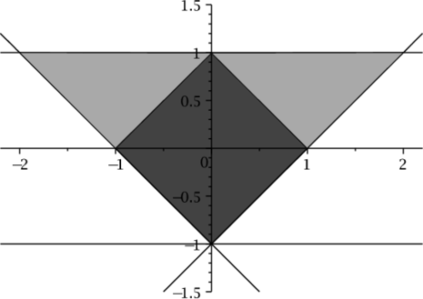
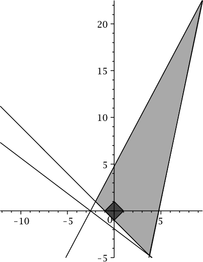
Solution of \eqref{eqintshura2} are graphically compared to with set of pairs $(\alpha_1, \alpha_2)$ satisfying \eqref{estLiang2002} in Figure 3 a).
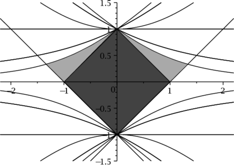
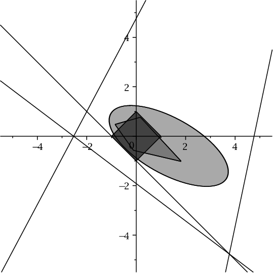
To clarify the dependence on $t_i$ we present in Figure 3 b) similar comparison for $t_1=3,\ t_2=8$.
Our approach apparently gives more general conditions than \eqref{estLiang2002} or its particular case from the works of Byszewski, even though we made sufficient conditions \eqref{eqintshura2} independent on $\theta_0$.
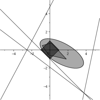
Propostion 2 of Theorem 3 ought to be more advantageous for operator coefficients with smaller $\theta$. Let us fix $\theta_0 =\pi/3$. We get $$ O_1 = 0.3950734246 , \quad r = 0.6049265754 $$ for the parameters of encompassing circle and $$ \begin{array}{ll} P_1(z’) &\approx 0.37 \alpha_2 {z’}^2+(0.6 \alpha_1+0.48 \alpha_2) z’+1+0.4 \alpha_1+0.16 \alpha_2 , \\ P_2(z’') &\approx \alpha_2 {z’'}^2+(\alpha_1+0.79 \alpha_2) {z’'}+1+0.4 \alpha_1+0.16 \alpha_2 \end{array} $$ for polynomials \eqref{zerosPol1}, \eqref{zerosPol2} correspondingly.
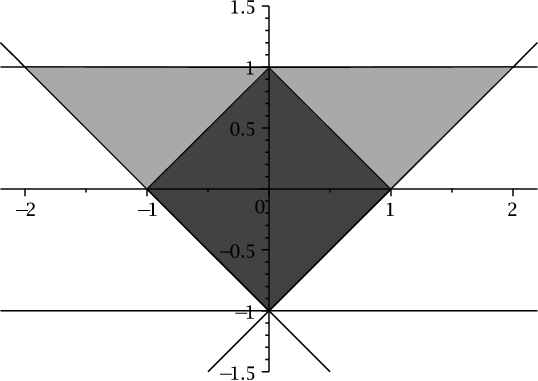
Application of the mentioned proposition along with \eqref{shurCrit} (setting $t_1=1,\ t_2=2$ as before) gives us the set of admissible $(\alpha_1,\alpha_2)$ depicted in Figure 4. One can see that this set contains both admissible parameters sets obtained from proposition 1 of the same theorem and condition \eqref{estLiang2002}.
Materials
Figures
Codes
- Maple file circumcircle_and_preimage.mws to generate Figure 1
- Maple file 1pnc_alpha_complex.mws to generate Figure 2
- Maple file 2pnc_tShura_alpha_real.mws to generate Figure 3
- This code implements root-free region tests presented in Lemmas 1—4, Shur-Cohn algorithm and encompassing circle parameters calculation. It allows to obtain inequalities for admissible parameters sets based on the various propositions of Theorem 2.